
Introduction
xlOptimizer fully implements Differential Evolution (DE), a relatively new stochastic method which has attracted the attention of the scientific community. DE was introduced by Storn and Price [1] and has approximately the same age as PSO. An early version was initially conceived under the term “Genetic Annealing” and published in a programmer’s magazine [2]. The DE algorithm is extremely simple; the uncondensed C-style pseudocode of the algorithm spans less than 25 lines [2].
How does it work?
Differential evolution bears no natural paradigm, i.e. it is not biologically inspired. It is an evolutionary algorithm which evolves a population of possible solutions. Basically, DE adds the weighted difference between two population members to a third member. This simple idea has proved to be an extremely effective method of optimization.
Mathematical formulation
According to the classic version of DE, a population of p individuals is randomly dispersed within the design space. The population is denoted as Px,g, as follows:
\[\begin{gathered}
{{\mathbf{x}}_L} \leqslant {{\mathbf{x}}_{i,0}} \leqslant {{\mathbf{x}}_U}{\text{ }}\forall i \in \left\{ {1,2,...,P} \right\} \hfill \\
{{\mathbf{P}}_{{\mathbf{x}},g}} = \left( {{{\mathbf{x}}_{i,g}}} \right),{\text{ }}i \in \left\{ {1,2,...,P} \right\},{\text{ }}g \in \left\{ {0,1,...,{g_{\max }}} \right\} \hfill \\
{{\mathbf{x}}_{i,g}} = \left( {{x_{j,i,g}}} \right),{\text{ }}j \in \left\{ {1,2,...,D} \right\}. \hfill \\
\end{gathered} \]
where, Px,g= array of p vectors (individuals), xi,g= Np–dimensional vector representing a solution, i=index for vectors, g=index for generations, j=index for design variables, gmax=maximum number of generations and the parentheses indicate an array. At each evolutionary step (generation), a mutated population Pv,g is formed based on the current population Px,g, as follows:
\[{{\mathbf{v}}_{i,g}} = {{\mathbf{x}}_{r0,g}} + F\left( {{{\mathbf{x}}_{r1,g}} - {{\mathbf{x}}_{r2,g}}} \right)\]
where, r0, r1, r2 are random indices in {0,1,…,p-1} and F is a scalar DE algorithm parameter. Next, a trial population Pu,g is formed, as follows:
\[{{\mathbf{u}}_{i,g}} = \left( {{u_{j,i,g}}} \right) = \left\{ {\begin{array}{*{20}{c}}
{{v_{j,i,g}},{\text{ if }}\left( {r \leqslant {C_r}{\text{ or }}j = {j_{rand}}} \right)} \\
{{x_{j,i,g}},{\text{ otherwise}}}
\end{array}} \right.\]
where, randj = random number with uniform distribution in (0,1) that is sampled anew each time, jrand is a random index in {0,1,…,p-1} that ensures that at least one design variable will originate from the mutant vector, and Cr is a scalar DE algorithm parameter in the range (0,1]. The final step is the selection criterion, which is greedy. In case of a minimization problem:
\[{{\mathbf{x}}_{i,g + 1}} = \left\{ {\begin{array}{*{20}{c}}
{{{\mathbf{u}}_{i,g}},{\text{ if }}f\left( {{{\mathbf{u}}_{i,g}}} \right) \leqslant f\left( {{{\mathbf{x}}_{i,g}}} \right)} \\
{{{\mathbf{x}}_{i,g}},{\text{ otherwise}}}
\end{array}} \right.\]
The aforementioned formulation corresponds to the classic DE variant, denoted “rand/1/bin” [2], where “rand” indicates that base vectors are randomly chosen, “1” means that only one vector difference is used to form the mutated population, and the term “bin” (from binomial distribution) indicates that uniform crossover is employed during the formation of the trial population. A more greedy version is “best/1/bin” [2], where “best” indicates that the base vector used is the currently best vector in the population. Thus, the mutated population Pv,g is formed based on:
\[{{\mathbf{v}}_{i,g}} = {{\mathbf{x}}_{best,g}} + F\left( {{{\mathbf{x}}_{r1,g}} - {{\mathbf{x}}_{r2,g}}} \right)\]
In addition, “jitter” may be introduced to the parameter F and the previous equation is modified as follows:
\[\begin{gathered}
{{\mathbf{v}}_{i,g}} = {{\mathbf{x}}_{best,g}} + {F_j}\left( {{{\mathbf{x}}_{r1,g}} - {{\mathbf{x}}_{r2,g}}} \right) \hfill \\
{F_j} = F + d\left( {r - 0.5} \right) \hfill \\
\end{gathered} \]
where, randj = random number with uniform distribution in (0,1) that is sampled anew each time and d is the magnitude of the jitter.
The present variant is denoted as “rand-best/1/bin”. This variant was presented in [3] and it is a mix of the “rand/1/bin” and “best/1/bin” variants. Define rb as the expected ratio of evaluations with “rand/1/bin” as opposed to the ones with “best/1/bin”. If randj < rb, then evolution is carried out according to “rand/1/bin”. In the opposite case, “best/1/bin” is employed. Usual value of rb is 0.25. This variant was shown to combine the impressive initial performance of “best/1/bin” with the fine-tuning abilities of “rand/1/bin” [3].
Usual parameter values are the following: (a) p=30-50 vectors, (b) F=0.5, (c) Cr=0.9 (d) d=0.001 [3].
Options in xlOptimizer add-in
The following options are available in xlOptimizer add-in. Note that whenever an asterisk (*) is indicated in a text field, this means that the field accepts a formula rather than a certain value. The formula is identical to Microsoft Excel's formulas, without the preceding equal sign '='. Also, the function arguments are always separated by comma ',' while the dot '.' is used as a decimal point.
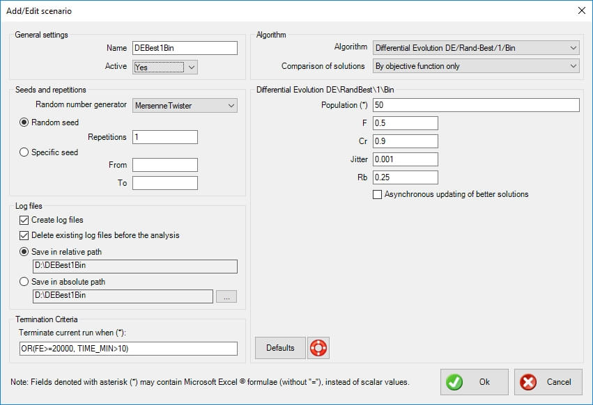
General settings
- Name: the name of the scenario to be run. It should be descriptive but also concise, as a folder with the same name will be (optionally) created, which will hold the log files for further statistical analysis.
- Active: select whether the scenario is active or not. If it is active, it will be run in sequence with the other active scenaria. In the opposite case, it will be ignored. This is very helpful when you experiment with settings.
Seeds and repetitions
Metaheuristic algorithms are based on random number generators. These are algorithms that produce a different sequence of random numbers for each seed they begin with. A seed is just an integer, and a different seed will produce a different evolution history with a different outcome. Robust metaheuristic algorithms should, on average, perform the same no matter what the seed is.
- Random number generator: select the random number generator to be used. The Mersenne Twister is default. The following options are available:
- NumericalRecipes: Numerical Recipes' [3] long period random number generator of L’Ecuyer with Bays-Durham shuffle and added safeguards
- SystemRandomSource: Wraps the .NET System.Random to provide thread-safety
- CryptoRandomSource: Wraps the .NET RNGCryptoServiceProvider
- MersenneTwister: Mersenne Twister 19937 generator
- Xorshift: Multiply-with-carry XOR-shift generator
- Mcg31m1: Multiplicative congruential generator using a modulus of 2^31-1 and a multiplier of 1132489760
- Mcg59: Multiplicative congruential generator using a modulus of 2^59 and a multiplier of 13^13
- WH1982: Wichmann-Hill's 1982 combined multiplicative congruential generator
- WH2006: Wichmann-Hill's 2006 combined multiplicative congruential generator
- Mrg32k3a: 32-bit combined multiple recursive generator with 2 components of order 3
- Palf: Parallel Additive Lagged Fibonacci generator
- Random repetitions: use this option if you wish the program to select random seeds for every run. Also, select the number of repetitions. If you wish to perform a statistical analysis of the results, a sample of 30 runs should be sufficient.
- Specific seed: use this option if you wish to use a selected range of integers as seeds. Note that seeds are usually large negative integers.
Log files
- Create log files: select whether you wish to create a log file for each run. This is imperative if you wish to statistically analyze the results. If you are only interested in the best result out of a certain number of runs, disabling this will increase performance (somewhat).
- Delete existing log files before the analysis: select this option if you want the program to delete all existing (old) log files (with the extension ".output") in the specific folder, before the analysis is performed.
- Save in relative path: select this option to create and use a folder relative to the spreadsheet's path. The name of the folder is controlled in the General Settings > Name.
- Save in absolute path: select this option to create and use a custom folder. Press the corresponding button with the ellipses "..." to select the folder.
Termination criteria
Each scenario needs a specific set of termination criteria. You can use an excel-like expression with the following variables (case insensitive):
- 'BEST_1', 'BEST_2', etc represent the best value of the objective function 1, 2, etc in the population.
- 'AVERAGE_1', 'AVERAGE_2', etc represent the average value of the objective function 1, 2, etc in the population.
- 'WORST_1', 'WORST_2', etc represent the worst value of the objective function 1, 2, etc in the population.
- 'MIN_1', 'MIN_2', etc represent the minimum value of the objective function 1, 2, etc in the population.
- 'MAX_1', 'MAX_2', etc represent the maximum value of the objective function 1, 2, etc in the population.
- 'FE' represents the function evaluations so far.
- 'TIME_MIN' represents the elapsed time (in minutes) since the beginning of the run.
- 'BEST_REMAINS_FE' represents the number of the last function evaluations during which the best solution has not been improved.
The default formula is 'OR(FE>=20000, TIME_MIN>10)' which means that the run is terminated when the number of function evaluations is more than 20000 or the run has lasted more than 10 minutes.
Algorithm
- Algorithm: select the algorithm to be used in the specific scenario. In this case 'Differential Evolution DE/rand/1/bin' is selected.
- Comparison of solutions: select whether feasibility (i.e. the fact that a specific solution does not violate any constraints) is used in the comparison between solutions. The following options are available:
- By objective function only: feasibility is ignored, and only the objective function (potentially including penalties from constraint violations) is used to compare solutions.
- By objective function and feasibility: the objective function (potentially including penalties from constraint violations) is used to compare solutions, but in the end, a feasible solution is always preferred to an infeasible one.
Differential Evolution DE/rand/1/bin
The following options are specific to Differential Evolution DE/rand/1/bin.
Population
Enter a formula for the calculation of the population size. You can use an excel-like expression with the following variables (case insensitive):
- 'VARS' represents the number of variables (i.e. the dimensionality of the problem).
The default setting is '50', which is a good choice for most problems.
F
Select an appropriate value for the parameter F. The default setting is 0.5.
Cr
Select an appropriate value for the parameter Cr (between 0 and 1). Small values are expected to work better with separable problems. The default setting is 0.9.
Jitter
Select an appropriate level for the jitter. This is used to maintain diversity, as the base vector is always the currently best in the population. The default setting is 0.001.
Rb
Select an appropriate value for Rb. Higher values produce more robust results (closer to rand/1/bin), while small values are more greedy (closer to best/1/bin). The default setting is 0.25, but this should work well only with unimodal problems. If you suspect multimodality, a higher value e.g. 0.8 should be more appropriate.
Asynchronous updating of better solutions
Select this option if you wish the comparison between trial and existing vector to take place within the inner loop. This means that the better solution will be available for mutation within the current generation. If this is unchecked, all trial vectors are formed at the end of the loop (which is the standard).
References
[1] R. Storn, K. Price, “Differential Evolution – A Simple and Efficient Heuristic for Global Optimization over Continuous Spaces”, Journal of Global Optimization, 11, 341 359, 1997.
[2] R. Storn, K. Price, J.A. Lampinen, “Differential Evolution – a practical approach to global optimization”, Springer, 2005.
[3] Charalampakis, A. E., Dimou, C. K., “Comparison of Evolutionary Algorithms for the Identification of Bouc-Wen Hysteretic Systems”, Journal of Computing in Civil Engineering, ASCE, (2013) doi:10.1061/(ASCE)CP.1943-5487.0000348.